Split Worksheet in Excel

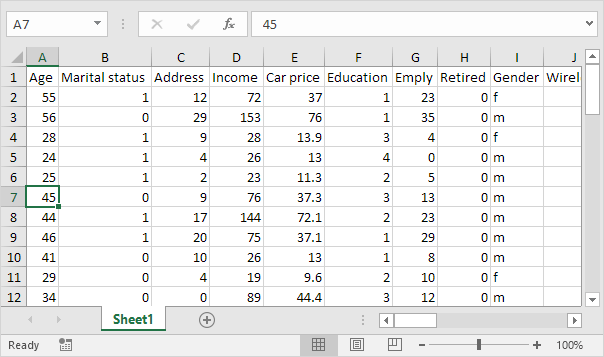
You can split your Excel worksheet into panes to view multiple distant parts of your worksheet at once. Simply use the split bar to change the size of each pane.

Split Horizontally

To split your worksheet (window) into an upper and lower part (pane) execute the following steps.

1. First select a cell in column A.

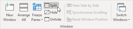
2. On the View tab in the Window group click Split.

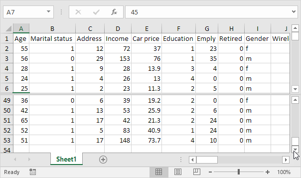
3. Notice the two vertical scroll bars. For example use the lower vertical scroll bar to move to row 49. As you can see the first 6 rows remain visible.

4. To change the window layout use the horizontal split bar that divides the panes.

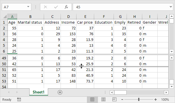
Note: to remove the split simply double click the split bar.

Split Vertically

To split your sheet into a left and right pane execute the following steps.

1. First select a cell in row 1.

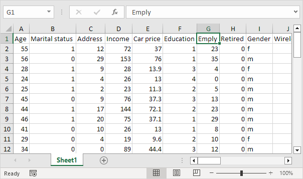
2. On the View tab in the Window group click Split.

Tip: you can also use the shortcut Alt + W + S to quickly enable or disable split screen in Excel.

Result:

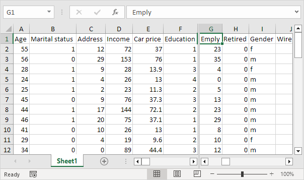
Conclusion: you'll have two horizontal scroll bars after splitting your worksheet vertically.

Split into Four Panes

You can even split your sheet into four panes. To achieve this execute the following steps.

1. First select a cell that is not in column A or row 1.

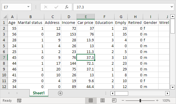
2. On the View tab in the Window group click Split.

Result:

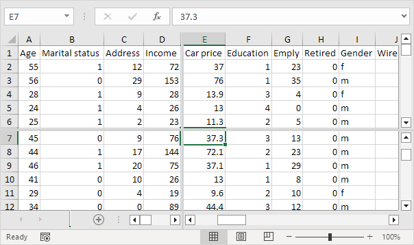
Note: any changes you make to one pane are immediately reflected in the other panes.