Custom Number Format in Excel

Excel has many built-in formats that you can use: Currency Accounting Date Time Percentage etc. If you cannot find the right format you can create a custom number format.

Leading Zeros

For example you might have codes that consist of 5 numbers. Instead of typing 00041 simply type 41 and let Excel add the leading zeros.

1. Enter the value 41 into cell A1.

2. Select cell A1 right click and then click Format Cells.

3. Select Custom.

4. Type the following number format code: 00000

5. Click OK.

Note: Excel gives you a live preview of how the number will be formatted (under Sample).

Result:

Note: cell A1 still contains the number 41. We only changed the appearance of this number not the number itself.

Decimal Places

You can also control the number of decimal places. Use 0 to display the nearest integer value. Use 0.0 for one decimal place. Use 0.00 for two decimal places etc.

1. Enter the value 839.1274 into cell A1.

2. Use the following number format code: 0.00

Add Text

You can also add text to your numbers. For example add "ft".

1. Enter the value 839.1274 into cell A1.

2. Use the following number format code: 0.0 "ft"

Note: remember we only changed the appearance of this number not the number itself. You can still use this number in your calculations.

Large Numbers

You can also control large numbers. Use one comma () to display thousands and use two commas () to display millions.

1. Enter the following values in cells A1 B1 C1 and D1: 1000000 2500000 81000000 and 700000.

2. Use the following number format code: 0.0 "M"

Note: we used 0.0 for one decimal place and "M" to add the letter M.

Repeat Characters

Use the asterisk (*) followed with a character to fill a cell with that character.

1. Type Hi into cell A1.

2. Use the following number format code: @ *-

Note: the @ symbol is used to get the text input.

Colors

You can control positive numbers negative numbers zero values and text all at the same time! Each part is separated with a semicolon (;) in your number format code.

1. Enter the following values in cells A1 B1 C1 and A2: 5000000 0 Hi and -5.89.

2. Use the number format code: [Green]$###0_);[Red]$(###0);"zero";[Blue]"Text:" @

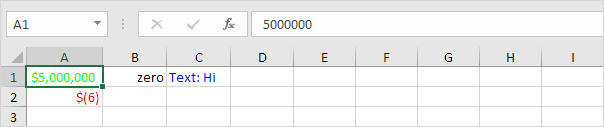
Note: ### is used to add commas to large numbers. To add a space use the underscore "_" followed by a character. The length of the space will be the length of this character. In our example we added a parenthesis ")". As a result the positive number lines up correctly with the negative number enclosed in parentheses. Use two parts separated with a semicolon (;) to control positive and negative numbers only. Use three parts separated with a semicolon (;) to control positive numbers negative numbers and zero values only.

Dates and Times

You can also control dates and times. Use one of the existing Date or Time formats as a starting point.

1. Enter the value 42855 into cell A1.

2. Select cell A1 right click and then click Format Cells.

3. Select Date and select the Long Date.

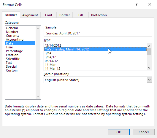
Note: Excel gives you a live preview of how the number will be formatted (under Sample).

4. Select Custom.

5. Slightly change the number format code to: mm/dd/yyyy dddd

6. Click OK.

Result:

General note: a custom number format is stored in the workbook where you create it. If you copy a value with a custom number format to another workbook it will also be available in that workbook.