Table of Contents
Transpose
Use the ‘Paste Special Transpose‘ option to switch rows to columns or columns to rows in Excel. You can also use the TRANSPOSE function.
Paste Special Transpose
To transpose data execute the following steps.
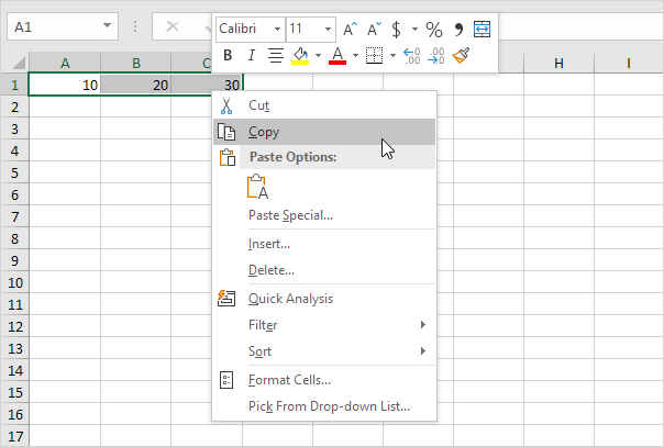
1. Select the range A1:C1.
2. Right click and then click Copy.
3. Select cell E2.
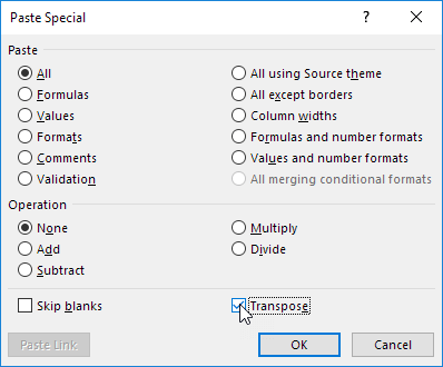
4. Right click and then click Paste Special.
5. Check Transpose.
6. Click OK.
TRANSPOSE function
To insert the TRANSPOSE function execute the following steps.
1. First select the new range of cells.
2. Type in =TRANSPOSE(
3. Select the range A1:C1 and close with a parenthesis.
4. Finish by pressing CTRL + SHIFT + ENTER.
Note: the formula bar indicates that this is an array formula by enclosing it in curly braces {}. To delete this array formula select the range E2:E4 and press Delete.
5. If you have Excel 365 or Excel 2021 simply select cell E2 enter the TRANSPOSE function and press Enter. Bye bye curly braces.
Note: the TRANSPOSE function entered into cell E2 fills multiple cells. Wow! This behavior in Excel 365/2021 is called spilling.
Transpose Table without Zeros
The TRANSPOSE function in Excel converts blank cells to zeros. Simply use the IF function to fix this problem.
1. For example cell B4 below is blank. The TRANSPOSE function converts this blank cell to a zero (cell G3).
2. If blank the IF function below returns an empty string (two double quotes with nothing in between) to transpose.
Transpose Magic
The ‘Paste Special Transpose’ option is a great way to transpose data but if you want to link the source cells to the target cells you need a few magic tricks.
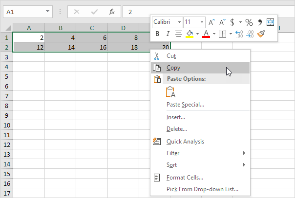
1. Select the range A1:E2.
2. Right click and then click Copy.
3. Select cell A4.
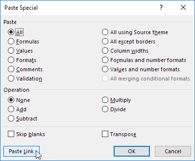
4. Right click and then click Paste Special.
5. Click Paste Link.
Result:
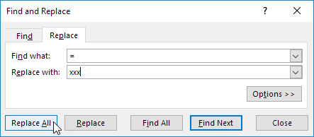
6. Select the range A4:E5 and replace all equal signs with xxx.
Result:
7. Use ‘Paste Special Transpose’ to transpose this data.
8. Select the range G1:H5 and replace all occurrences of ‘xxx’ with equal signs (the exact opposite of step 6).
Note: for example change the value in cell C2 from 16 to 36. The value in cell H3 will also change from 16 to 36.
