Table of Contents
Strikethrough
This example teaches you how to apply strikethrough formatting in Excel. You can still read text with a strikethrough effect.
1. For example select the range A2:A4.
2. Right click and then click Format Cells (or press Ctrl + 1).
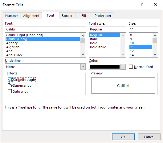
The ‘Format Cells’ dialog box appears.
3. On the Font tab under Effects click Strikethrough.
4. Click OK.
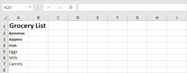
Result:
You can also use a keyboard shortcut to quickly apply strikethrough formatting in Excel.
5. For example select cell A7.
6. Press Ctrl + 5.
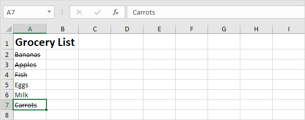
Result:
Note: simply press Ctrl + 5 again to remove the strikethrough effect. There’s no double strikethrough option in Excel.
7. To apply strikethrough formatting to just part of a cell first select the text in the formula bar.
8. Press Ctrl + 5.
Let’s take a look at 2 more cool ways to quickly apply strikethrough formatting in Excel.
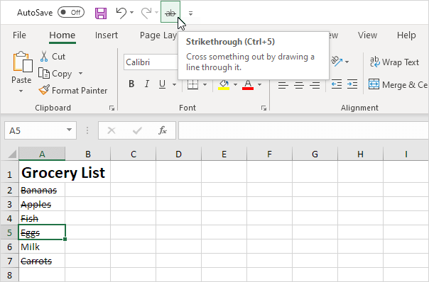
9. Add a strikethrough button to the Quick Access Toolbar.
10. Select cell A5 and click the strikethrough button.
11. Add the following code lines to the BeforeDoubleClick Event:
Target.Font.Strikethrough = True
Cancel = True
12. Double click cell A6.
Note: try it yourself. Download the Excel file use the strikethrough button or double click a cell to quickly apply strikethrough formatting.


