Table of Contents
ISERROR
This example illustrates the ISERROR function in Excel.
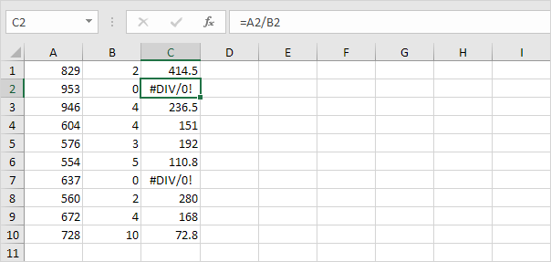
1. For example Excel displays the #DIV/0! error when a formula tries to divide a number by 0.
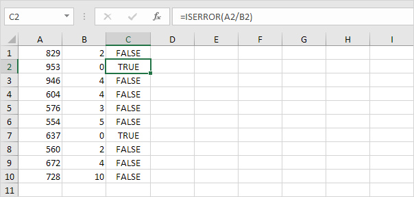
2. The ISERROR function in Excel checks whether a value is an error and returns TRUE or FALSE.
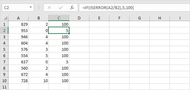
3. Add the IF function. If a cell contains an error the value 5 is returned. If not the value 100 is returned.
4. Use the IFERROR function to return the result of a formula (if there’s no error) or an alternative result such as text (if there’s an error).
5. Use COUNT IF and ISERROR to count the total number of errors in a range of cells.
Note: finish an array formula by pressing CTRL + SHIFT + ENTER. Excel adds the curly braces {}. In Excel 365 or Excel 2021 finish by simply pressing Enter. You won’t see curly braces. Visit our page about Counting Errors for detailed instructions on how to create this array formula.


