Table of Contents
Reverse List
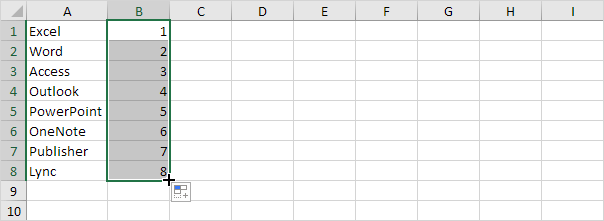
This article teaches you how to reverse the order of a list in Excel. For example we want to reverse the list in column A below.
1. Enter the value 1 into cell B1 and the value 2 into cell B2.
2. Select the range B1:B2 click the lower right corner of this range and drag it down to cell B8.
3. Click any number in the list in column B.
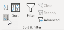
4. To sort in descending order on the Data tab in the Sort & Filter group click ZA.
Result: not only the list in column B but also the list in column A has been reversed.
If you have Excel 365 or Excel 2021 use SEQUENCE SORTBY and ROWS to sort a list in reverse order. The following formula is pretty awesome.
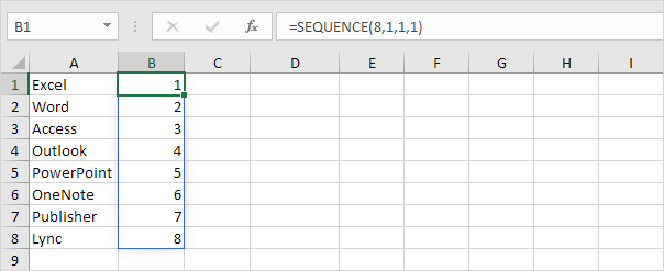
5. First use the SEQUENCE function to generate a list of numbers. The SEQUENCE function below has 4 arguments. Rows = 8 Columns = 1 Start = 1 Step = 1.
Note: the SEQUENCE function entered into cell B1 fills multiple cells. Wow! This behavior in Excel 365/2021 is called spilling.
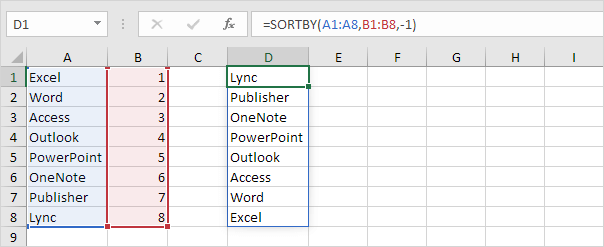
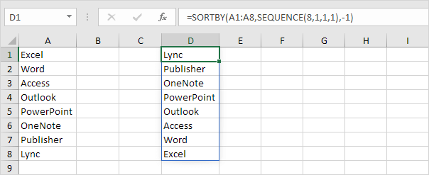
6. The SORTBY function sorts a range based on the values in a corresponding range. Use -1 (third argument) to sort in descending order.
7. Nest the SEQUENCE function inside the SORTBY function.
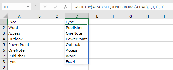
8. If you have a longer list of say 20 names change the value 8 to 20 in the formula shown above or even better use the ROWS function.
Note: the ROWS function simply counts the number of rows in a range.
