Table of Contents
Gantt Chart
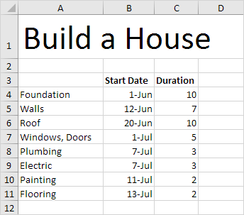
Excel does not offer Gantt as a chart type but it’s easy to create a Gantt chart by customizing the stacked bar chart type. Below you can find our Gantt chart data.
To create a Gantt chart execute the following steps.
1. Select the range A3:C11.
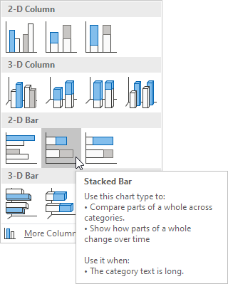
2. On the Insert tab in the Charts group click the Column symbol.
3. Click Stacked Bar.
Result:
4. Enter a title by clicking on Chart Title. For example Build a House.
5. Click the legend at the bottom and press Delete.
6. The tasks (Foundation Walls etc.) are in reverse order. Right click the tasks on the chart click Format Axis and check ‘Categories in reverse order’.
Result:
7. Right click the blue bars click Format Data Series Fill & Line icon Fill No fill.
8. Dates and times are stored as numbers in Excel and count the number of days since January 0 1900. 1-jun-2017 (start) is the same as 42887. 15-jul-2017 (end) is the same as 42931. Right click the dates on the chart click Format Axis and fix the minimum bound to 42887 maximum bound to 42931 and Major unit to 7.
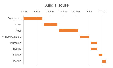
Result: a Gantt chart in Excel.
Note that the plumbing and electrical work can be executed simultaneously.


