Table of Contents
Loan Calculator
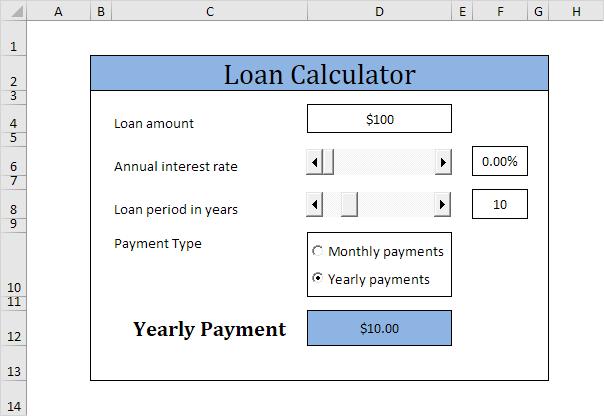
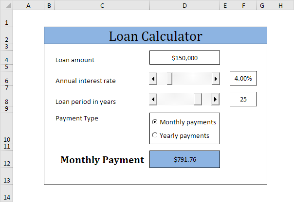
This page teaches you how to create a simple loan calculator in Excel VBA. The worksheet contains the following ActiveX controls: two scrollbars and two option buttons.
Note: the instructions below do not teach you how to format the worksheet. We assume that you know how to change font types insert rows and columns add borders change background colors etc.
Execute the following steps to create the loan calculator:
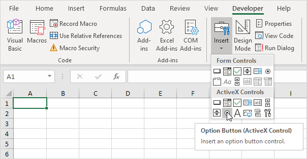
1. Add the two scrollbar controls. Click on Insert from the Developer tab and then click on Scroll Bar in the ActiveX Controls section.
2. Add the two option buttons. Click on Insert from the Developer tab and then click on Option Button in the ActiveX Controls section.
Change the following properties of the scrollbar controls (make sure Design Mode is selected).
3. Right mouse click on the first scrollbar control and then click on Properties. Set Min to 0 Max to 20 SmallChange to 0 and LargeChange to 2.
4. Right mouse click on the second scrollbar control and then click on Properties. Set Min to 5 Max to 30 SmallChange to 1 LargeChange to 5 and LinkedCell to F8.
Explanation: when you click on the arrow the scrollbar value goes up or down by SmallChange. When you click between the slider and the arrow the scrollbar value goes up or down by LargeChange.
Create a Worksheet Change Event. Code added to the Worksheet Change Event will be executed by Excel VBA when you change a cell on a worksheet.
5. Open the Visual Basic Editor.
6. Double click on Sheet1 (Sheet1) in the Project Explorer.
7. Choose Worksheet from the left drop-down list and choose Change from the right drop-down list.
8. The Worksheet Change Event listens to all changes on Sheet1. We only want Excel VBA to run the Calculate sub if something changes in cell D4. To achieve this add the following code line to the Worksheet Change Event (more about the Calculate sub later on).
If Target.Address = “$D$4” Then Application.Run “Calculate”
9. Get the right percentage in cell F6 (change the format of cell F6 to percentage). Right mouse click on the first scrollbar control and then click on View Code. Add the following code lines:
Private Sub ScrollBar1_Change()
Range(“F6”).Value = ScrollBar1.Value / 100
Application.Run “Calculate”
End Sub
10. Right mouse click on the second scrollbar control and then click on View Code. Add the following code line:
Private Sub ScrollBar2_Change()
Application.Run “Calculate”
End Sub
11. Right mouse click on the first option button control and then click on View Code. Add the following code line:
Private Sub OptionButton1_Click()
If OptionButton1.Value = True Then Range(“C12”).Value = “Monthly Payment”
Application.Run “Calculate”
End Sub
12. Right mouse click on the second option button control and then click on View Code. Add the following code line:
Private Sub OptionButton2_Click()
If OptionButton2.Value = True Then Range(“C12”).Value = “Yearly Payment”
Application.Run “Calculate”
End Sub
13. Time to create the sub. You can go through our Function and Sub chapter to learn more about subs. If you are in a hurry simply place the sub named Calculate into a module (In the Visual Basic Editor click Insert Module).
Sub Calculate()
Dim loan As Long rate As Double nper As Integer
loan = Range(“D4”).Value
rate = Range(“F6”).Value
nper = Range(“F8”).Value
If Sheet1.OptionButton1.Value = True Then
rate = rate / 12
nper = nper * 12
End If
Range(“D12”).Value = -1 * WorksheetFunction.Pmt(rate nper loan)
End Sub
Explanation: the sub gets the right parameters for the worksheet function Pmt. The PMT function in Excel calculates the payments for a loan based on constant payments and a constant interest rate. If you make monthly payments (Sheet1.OptionButton1.Value = True) Excel VBA uses rate / 12 for rate and nper *12 for nper (total number of payments). The result is a negative number because payments are considered a debit. Multiplying the result by -1 gives a positive result.


